Different Performance Metrics in Machine Learning

To check the performance of the models we use performance matrices means how good our model is. there are different-different types of performance matrices for classification and regression algorithms. 

1. for the classification algorithms

a) Accuracy     b) Confusion Matrix      c) ROC & AUC      d)  Log loss

2. for the regression algorithms 

a) R-Square   b) adjusted- R - Square

1. a) Accuracy: Accuracy is one of the performance measures that is used to check the performance of the model like how good our model is. It is one of the easy-to-understand measures. It lies between 0 and 1. Here 0 means the model is bad and 1 means the model is good.

                                           Accuracy is defined as = no. of correctly classified pts/total no. of pts in Dtest

But there are some conditions where Accuracy can not be used as a performance matrix that is :

Case1. When we have an imbalanced dataset: Imagine we have an imbalance dataset in that 90% of data is -ive and 10% of data is +ive. Now we have a dump model so it will give the result according to the majority vote.
So if we pass any query point it will always give -ive output. So when we check the accuracy of this then it will be 90% which is very good but this is good because in our dataset we have 90% pts -ive so 90% times the output will be correct.
That’s why if we have an imbalanced dataset then we should not use accuracy as a performance measure.

Case2. When our model gives the probability scores:  Suppose we have 4 pts in that 2 are +ive and 2 are -ive. And we have two models M1 and M2 that gives a probability score as an output. Now, we define that if the probability score is less than 0.5 then in terms of classification, the output will be 0 (means bad model) and if it is greater than 0.5 then the output will be 1(good model). So in this case one model is giving prob. Score 0.55(M1) and the other is giving 0.95(M2) now if we calculate the accuracy of both the models then it will be the same for both but we know M2 is much better than M1.  That’s why in this case, accuracy is not a good measure to check performance.

1. b) Confusion Matrix:  A confusion matrix is a matrix that is used to check the performance of the models. It is used to summarise the performance of the classification algorithm. using the confusion matrix we can find the TPR, TNR, FPR, FNR, precision, recall, and F-1 Score.

Since in the case of the imbalanced dataset, we can’t use accuracy but use TPR(True Positive Rate), TNR(True Negative Rate), FNR(False Negative Rate), FPR(False Positive Rate) gives much more sensible results.

In binary classification, every cell has a special name. Each cell value is the total number of points. above is the confusion matrix for binary classification (see above figure1).

From figure1: 0 is negative and 1 is positive. And is read as T means are you correct and N means what is the predicted label. (TP+FN) is equal to actual total positives (P) and (FP+TN) is equal to the actual total negatives. Similarly, we can make a confusion matrix for multi-classification.

Precision:- Precision is defined as of all the positive points the model predicted to be +ive, what percentage of them are actually positive. Or we can say precision is the ratio of true positives and all the positives.

F-1 Score:- it is the combination of precision and recall or we can say it is a trade-off between precision and recall. it lies between 0 and 1.
             
                                                                                                                      F-1 Score = (2*Precision*recall) / (precision+recall)

This means if the F-1 Score is high then precision and recall will also be high.

1. c) ROC & AUC: ROC is a receiver operating characteristic curve and the area under this ROC curve is known as AUC.these are other performance matrices. This value ranges from 0 t 1. It is mainly used for binary classification problems.it works on probability scores.

there are some steps to calculate ROC and AUC:-
i). In the first step, we sort the data table based on the decreasing values of predictions (Y^).

ii). Thresholding: in this, the topmost value is selected as a threshold value and any value above or equal to this is marked as class1 and any value below this is marked as class 0.  For the different values of threshold, there will be different lists of predictions.

iii). Now, we calculate TPR, FPR for each of the lists of predictions. Now if our data has n rows then we will have n threshold values similarly n different TPR and FPR. Here the values of TPR, and FPR will lie between 0 and 1.

iv). Now we will plot FPR on the x-axis and TPR on the y-axis. By plotting these points we will get a curve that curve is called the ROC curve. And the total area under the curve is 1.

And the area under the ROC curve is called the area under the curve (AUC). its value ranges from 0 to 1. higher the value the better model is.

Now, other properties of AUC: 

 i). AUC is impacted by the imbalance dataset. Even a dumb model can have a high AUC.

ii). AUC for the random model will be 0.5. This means for each prediction it will select class 0 and class 1 with equal probability.

iii). We can also switch our predictions from 0 to 1 if we have a very low AUC Score.
For example, we have AUC is 0.2 then it will give the class label 0 then we can flip this class label from 0 to1 then the AUC score will be 1-0.2 = 0.8.which is a good AUC score.

For more understanding here above is the geometric explaination of ROC and AUC, to see which AUC and ROC values are good. here the dotted line is due to the random classifier that has an AUC value of 0.5 and a 1 AUC value is the Perfect classifier. An AUC value is less than 0.5 is a bad classifier and an AUC value greater than 0.5 is a good classifier.

1.d) Log-Loss: log loss is a loss matrix that lies between [0, infinite) . lower the loss value the better the model is. Log loss deals with the probability scores. It is a negative average of all the points.

In the formula, when y is equal to 1 then the second term of the formula will be zero and the remaining term will be the probability of y (target value) belonging to 1 then greater the value of y', the lower the loss will be.
This log-loss formula can also be extended to a multiclass setting.   Log-loss is defined as follows (see in the image):-

                                                                                          


2. a) R-square: R-squared statistic or the coefficient of determination is a scale-invariant statistic that gives the proportion of variation in the target variable explained by the linear regression model.  

                                    R-squared = (TSS-RSS)/TSS

                    = Explained variation/ Total variation

                    = 1 – Unexplained variation/ Total variation

So R-squared gives the degree of variability in the target variable that is explained by the model or the independent variables. If this value is 0.7, then it means that the independent variables explain 70% of the variation in the target variable.

R-squared value always lies between 0 and 1. A higher R-squared value indicates a higher amount of variability being explained by our model and vice-versa.

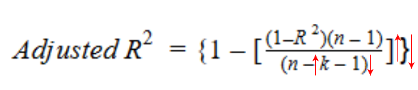
Let’s have a look at the formula for adjusted R-squared to better understand its working.

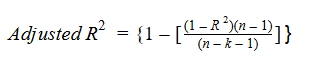Here,

• n represents the number of data points in our dataset
• k represents the number of independent variables, and
• R represents the R-squared values determined by the model.

So, if R-squared does not increase significantly on the addition of a new independent variable, then the value of Adjusted R-squared will actually decrease.