Linear Regression in Python

Introduction : This article attempts to be the reference you need when it comes to understanding and performing linear regression. Although the algorithm is simple, only a few truly understand the underlying principles.

First, we will dig deep into the theory of linear regression to understand its inner workings. Then, we will implement the algorithm in Python to model a business problem.

I hope this article finds its way to your bookmarks! For now, let’s get to it!

The Theory

How you’ll feel studying linear regression

Linear regression is probably the simplest approach for statistical learning. It is a good starting point for more advanced approaches, and in fact, many fancy statistical learning techniques can be seen as an extension of linear regression. Therefore, understanding this simple model will build a good base before moving on to more complex approaches.

Linear regression is very good to answer the following questions:

• Is there a relationship between 2 variables?
• How strong is the relationship?
• Which variable contributes the most?
• How accurately can we estimate the effect of each variable?
• How accurately can we predict the target?
• Is the relationship linear? (duh)
• Is there an interaction effect?

Estimating the coefficients

Let’s assume we only have one variable and one target. Then, linear regression is expressed as:

Equation for a linear model with 1 variable and 1 target

In the equation above, the betas are the coefficients. These coefficients are what we need in order to make predictions with our model.

So how do we find these parameters?

To find the parameters, we need to minimize the least squares or the sum of squared errors. Of course, the linear model is not perfect and it will not predict all the data accurately, meaning that there is a difference between the actual value and the prediction. The error is easily calculated with:

Subtract the prediction from the true value

But why are the errors squared?

We square the error, because the prediction can be either above or below the true value, resulting in a negative or positive difference respectively. If we did not square the errors, the sum of errors could decrease because of negative differences and not because the model is a good fit.

Also, squaring the errors penalizes large differences, and so the minimizing the squared errors “guarantees” a better model.

Let’s take a look at a graph to better understand.

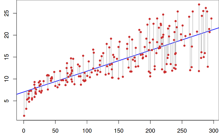
Linear fit to a data set

In the graph above, the red dots are the true data and the blue line is linear model. The grey lines illustrate the errors between the predicted and the true values. The blue line is thus the one that minimizes the sum of the squared length of the grey lines.

After some math that is too heavy for this article, you can finally estimate the coefficients with the following equations:

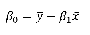
Where x bar and y bar represent the mean.

Estimate the relevancy of the coefficients

Now that you have coefficients, how can you tell if they are relevant to predict your target?

The best way is to find the p-value. The p-value is used to quantify statistical significance; it allows to tell whether the null hypothesis is to be rejected or not.

The null hypothesis?

For any modelling task, the hypothesis is that there is some correlation between the features and the target. The null hypothesis is therefore the opposite: there is no correlation between the features and the target.

So, finding the p-value for each coefficient will tell if the variable is statistically significant to predict the target. As a general rule of thumb, if the p-value is less than 0.05: there is a strong relationship between the variable and the target.

Assess the accuracy of the model

You found out that your variable was statistically significant by finding its p-value. Great!

Now, how do you know if your linear model is any good?

To assess that, we usually use the RSE (residual standard error) and the R² statistic.

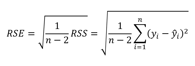
RSE formula

R² formula

The first error metric is simple to understand: the lower the residual errors, the better the model fits the data (in this case, the closer the data is to a linear relationship).

As for the R² metric, it measures the proportion of variability in the target that can be explained using a feature X. Therefore, assuming a linear relationship, if feature X can explain (predict) the target, then the proportion is high and the R² value will be close to 1. If the opposite is true, the R² value is then closer to 0.

The Theory of Multiple Linear Regression

In real life situations, there will never be a single feature to predict a target. So, do we perform linear regression on one feature at a time? Of course not. We simply perform multiple linear regression.

The equation is very similar to simple linear regression; simply add the number of predictors and their corresponding coefficients:

Multiple linear regression equation. p is the number of predictors

Assess the relevancy of a predictor

Previously, in simple linear regression, we assess the relevancy of a feature by finding its p-value.

In the case of multiple linear regression, we use another metric: the F-statistic.

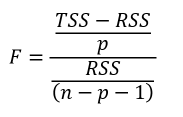
F-statistic formula. n is the number of data points and p is the number of predictors

Here, the F-statistic is calculated for the overall model, whereas the p-value is specific to each predictor. If there is a strong relationship, then F will be much larger than 1. Otherwise, it will be approximately equal to 1.

How larger than 1 is large enough?

This is hard to answer. Usually, if there is a large number of data points, F could be slightly larger than 1 and suggest a strong relationship. For small data sets, then the F value must be way larger than 1 to suggest a strong relationship.

Why can’t we use the p-value in this case?

Since we are fitting many predictors, we need to consider a case where there are a lot of features (p is large). With a very large amount of predictors, there will always be about 5% of them that will have, by chance, a very small p-value even though they are not statistically significant. Therefore, we use the F-statistic to avoid considering unimportant predictors as significant predictors.

Assess the accuracy of the model

Just like in simple linear regression, the R² can be used for multiple linear regression. However, know that adding more predictors will always increase the R² value, because the model will necessarily better fit the training data.

Yet, this does not mean it will perform well on test data (making predictions for unknown data points).

Adding interaction

Having multiple predictors in a linear model means that some predictors may have an influence on other predictors.

For example, you want to predict the salary of a person, knowing her age and number of years spent in school. Of course, the older the person, the more time that person could have spent in school. So how do we model this interaction effect?

Consider this very simple example with 2 predictors:

Interaction effect in multiple linear regression

As you can see, we simply multiply both predictors together and associate a new coefficient. Simplifying the formula, we see now that the coefficient is influenced by the value of another feature.

As a general rule, if we include the interaction model, we should include the individual effect of a feature, even if its p-value is not significant. This is known as the hierarchical principle. The rationale behind this is that if two predictors are interacting, then including their individual contribution will have a small impact on the model.

Alright! Now that we know how it works, let’s make it work! We will work through both a simple and multiple linear regression in Python and I will show how to assess the quality of the parameters and the overall model in both situations.

I strongly recommend that you follow and recreate the steps in your own Jupyter notebook to take full advantage of this tutorial.

Let’s get to it!

We all code like this, right?

Introduction

The data set contains information about money spent on advertisement and their generated sales. Money was spent on TV, radio and newspaper ads.

The objective is to use linear regression to understand how advertisement spending impacts sales.

Import libraries

The advantage of working with Python is that we have access to many libraries that allow us to rapidly read data, plot the data, and perform a linear regression.

I like to import all the necessary libraries on top of the notebook to keep everything organized. Import the following:

import pandas as pd
import numpy as npimport matplotlib.pyplot as pltfrom sklearn.linear_model import LinearRegression
from sklearn.metrics import r2_scoreimport statsmodels.api as sm

Read the data

Assuming that you downloaded the data set, place it in a data directory within your project folder. Then, read the data like so:

data = pd.read_csv("data/Advertising.csv")

To see what the data looks like, we do the following:

data.head()

And you should see this:

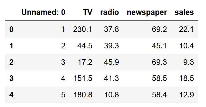
As you can see, the column Unnamed: 0 is redundant. Hence, we remove it.

data.drop(['Unnamed: 0'], axis=1)

Alright, our data is clean and ready for linear regression!

Simple Linear Regression

Modelling

For simple linear regression, let’s consider only the effect of TV ads on sales. Before jumping right into the modelling, let’s take a look at what the data looks like.

We use matplotlib , a popular Python plotting library to make a scatter plot.

plt.figure(figsize=(16, 8))
plt.scatter(
    data['TV'],
    data['sales'],
    c='black'
)
plt.xlabel("Money spent on TV ads ($)")
plt.ylabel("Sales ($)")
plt.show()

Run this cell of code and you should see this graph:

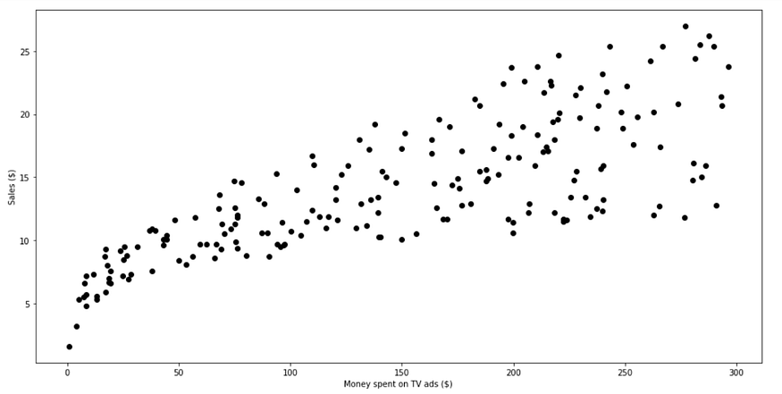
Scatter plot of money spent on TV ads and sales

As you can see, there is a clear relationship between the amount spent on TV ads and sales.

Let’s see how we can generate a linear approximation of this data.

X = data['TV'].values.reshape(-1,1)
y = data['sales'].values.reshape(-1,1)reg = LinearRegression()
reg.fit(X, y)print("The linear model is: Y = {:.5} + {:.5}X".format(reg.intercept_[0], reg.coef_[0][0]))

That’s it?

Yes! It is that simple to fit a straight line to the data set and see the parameters of the equation. In this case, we have

Simple linear regression equation

Let’s visualize how the line fits the data.

predictions = reg.predict(X)plt.figure(figsize=(16, 8))
plt.scatter(
    data['TV'],
    data['sales'],
    c='black'
)
plt.plot(
    data['TV'],
    predictions,
    c='blue',
    linewidth=2
)
plt.xlabel("Money spent on TV ads ($)")
plt.ylabel("Sales ($)")
plt.show()

And now, you see:

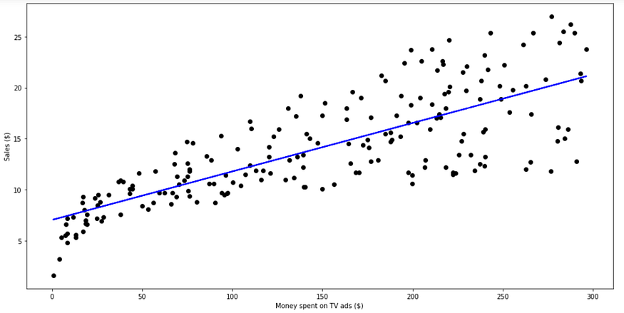
Linear fit

From the graph above, it seems that a simple linear regression can explain the general impact of amount spent on TV ads and sales.

Assessing the relevancy of the model

Now, if you remember the model is any good, we need to look at the R² value and the p-value from each coefficient.

Here’s how we do it:

X = data['TV']
y = data['sales']X2 = sm.add_constant(X)
est = sm.OLS(y, X2)
est2 = est.fit()
print(est2.summary())

Which gives you this lovely output:

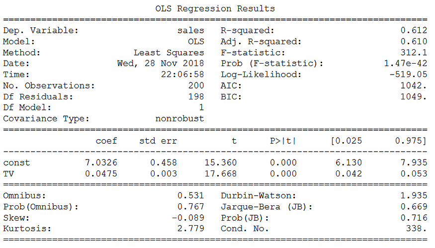
R² and p-value

Looking at both coefficients, we have a p-value that is very low (although it is probably not exactly 0). This means that there is a strong correlation between these coefficients and the target (Sales).

Then, looking at the R² value, we have 0.612. Therefore, about 60% of the variability of sales is explained by the amount spent on TV ads. This is okay, but definitely not the best we can to accurately predict the sales. Surely, spending on newspaper and radio ads must have a certain impact on sales.

Let’s see if a multiple linear regression will perform better.

Multiple Linear Regression

Modelling

Just like for simple linear regression, we will define our features and target variable and use scikit-learn library to perform linear regression.

Xs = data.drop(['sales', 'Unnamed: 0'], axis=1)
y = data['sales'].reshape(-1,1)reg = LinearRegression()
reg.fit(Xs, y)print("The linear model is: Y = {:.5} + {:.5}*TV + {:.5}*radio + {:.5}*newspaper".format(reg.intercept_[0], reg.coef_[0][0], reg.coef_[0][1], reg.coef_[0][2]))

Nothing more! From this code cell, we get the following equation:

Multiple linear regression equation

Of course, we cannot visualize the impact of all three mediums on sales, since it has a total of four dimensions.

Notice that the coefficient for newspaper is negative, but also fairly small. Is it relevant to our model? Let’s see by calculating the F-statistic, R² value and p-value for each coefficient.

Assessing the relevancy of the model

As you must expect, the procedure here is very similar to what we did in simple linear regression.

X = np.column_stack((data['TV'], data['radio'], data['newspaper']))
y = data['sales']X2 = sm.add_constant(X)
est = sm.OLS(y, X2)
est2 = est.fit()
print(est2.summary())

And you get the following:

R², p-value and F-statistic

As you can see, the R² is much higher than that of simple linear regression, with a value of 0.897!

Also, the F-statistic is 570.3. This is much greater than 1, and since our data set if fairly small (only 200 data points), it demonstrates that there is a strong relationship between ad spending and sales.

Finally, because we only have three predictors, we can consider their p-value to determine if they are relevant to the model or not. Of course, you notice that the third coefficient (the one for newspaper) has a large p-value. Therefore, ad spending on newspaper is not statistically significant. Removing that predictor would slightly reduce the R² value, but we might make better predictions.

Thank You !!  :)